Hello and welcome to the TTC blog. I've had a lot of fun this offseason putting this website together and am excited to finally take some time to write about the data instead of staring at numbers ensuring they're (mostly?) correct. I envision this blog centering around ABS topics with the occasional foray into other baseball related stories. My name is Nate Burke and my dad instilled in me a love for this game when I could hardly walk. I work as a data analyst. Since that's probably all you want to know about me I'm gonna stop the intro there.
Lets get right into it.
Evaluating the impact of ABS Challenges
There are two easy ways to evaluate the impact of a challenge or any other play in baseball. How many runs did it net, and how much closer to winning is that team? This post is going to discuss the run value side of things.
The way this has been done for many years now is by evaluating the change in game state. Popularized in The Book: Playing the Percentages in Baseball (2006, Tom Tango, Andrew Dolphin, Mitchel Lichtman) as a preliminary calculation for wOBA and the now ubiquitous wRC+, the Run Expectancy 24 Matrix evaluates changes in game state when taking the number of outs and combination of runners on base into account. From that chart we can see the marginal run impact of something like moving a runner from 1st base to 2nd base with 1 out in the inning. When additionally incorporating the count of the current at-bat, we can create a similar chart that has 288 states and evaluates the impact of each pitch.
-
3 out states [0, 1, 2]
-
8 runner on base states [bases empty, runner on 1st, runners on 1st and 2nd, bases loaded, etc]
-
12 count states [0-0, 0-1, 0-2, 1-0, 1-1, etc]
3x8x12 = 288 states that the game can be in at any point.
Calculating the RE288 Matrix
There are two ways to do this. One is more versatile mathematically, but both were very interesting the first time I read about them, so I'll explain both.
Approach 1: Just count what actually happened (Empirical approach)
This is the simplest approach. You go through every pitch thrown over a period of time and label each one with its state, like runner on first, 0 outs, and a 1-1 count. Then you look at how many runs the team actually ended up scoring by the end of that half inning. Lets say there were 50,000 pitches thrown in the bases empty, 0 outs, 0-0 count state. Sometimes the team scored 0 runs, sometimes 1, sometimes 3. You add up all the runs and divide by 50,000. That average is your run expectancy for that state and you do this math for each of the 288 states.
Approach 2: Simulate it with a model (Markov Chain + Monte Carlo approach)
Instead of looking at the final outcome, this method looks at how the game moves from one pitch to the next using real data.
For example, from a 0 out, no runners on, 1-1 count, the next pitch might result in:
1-2 count (strike) happens 46% of the time
2-1 count (ball) happens 34% of the time
Runner on first (usually meaning single but that's not the point here) happens 4.5% of the time
(etc)
You calculate all of these initial probabilities from real data. That web of states and probabilities is called a Markov chain.
Then you simulate. You start at a game state, roll the dice based on the probabilities, move to the next state, roll again, and keep going until the inning ends. You record how many runs scored. If you do this 500,000 times for each starting state you get a very reliable picture of not just the average run value for each state, but the full distribution of how likely it is for a team to score N runs from this point through the end of the inning, like saying there's a 60% chance of scoring 0 runs, 20% chance of 1 run, 12% chance of 2 runs. That distribution part is important for Win Expectancy and Leverage Index calculations, topics that I'll be making posts for in the near future. The simulation part here is called Monte Carlo.
Here's an interactive widget you can toy with to see what this calculation is doing:
Markov Chain Pitch Simulator
Walk through a half-inning pitch by pitch
Choose a starting state and click Throw Pitch to simulate an inning. Each pitch randomly follows the Markov chain transition probabilities derived from 2022–2025 Statcast data.
Current State
Empty, 0 out, 0-0
Run Expectancy
0.489
Runs Scored
0
The RE288 Matrix
Plotting out the average runs scored from each state gives us this chart:
RE288: Run Expectancy by Game State
Each cell shows the average number of runs a team is expected to score from that base/out/count state through the end of the half inning. Higher values (orange) indicate more valuable offensive situations.
| Bases | 0-0 | 0-1 | 0-2 | 1-0 | 1-1 | 1-2 | 2-0 | 2-1 | 2-2 | 3-0 | 3-1 | 3-2 |
|---|---|---|---|---|---|---|---|---|---|---|---|---|
| Empty | 0.489 | 0.456 | 0.406 | 0.525 | 0.478 | 0.431 | 0.591 | 0.529 | 0.466 | 0.724 | 0.642 | 0.565 |
| 1B | 0.885 | 0.820 | 0.751 | 0.940 | 0.867 | 0.778 | 1.031 | 0.941 | 0.849 | 1.224 | 1.105 | 1.003 |
| 2B | 1.112 | 1.054 | 0.969 | 1.164 | 1.093 | 0.997 | 1.250 | 1.147 | 1.052 | 1.373 | 1.278 | 1.157 |
| 3B | 1.363 | 1.302 | 1.230 | 1.400 | 1.333 | 1.241 | 1.454 | 1.389 | 1.305 | 1.574 | 1.491 | 1.423 |
| 1B-2B | 1.482 | 1.392 | 1.268 | 1.561 | 1.450 | 1.314 | 1.710 | 1.564 | 1.384 | 2.014 | 1.840 | 1.601 |
| 1B-3B | 1.786 | 1.708 | 1.587 | 1.810 | 1.726 | 1.622 | 1.911 | 1.805 | 1.690 | 2.107 | 1.921 | 1.802 |
| 2B-3B | 1.943 | 1.851 | 1.749 | 2.009 | 1.877 | 1.756 | 2.088 | 1.940 | 1.824 | 2.183 | 2.101 | 1.972 |
| Loaded | 2.302 | 2.196 | 2.030 | 2.369 | 2.260 | 2.088 | 2.528 | 2.394 | 2.193 | 2.811 | 2.629 | 2.472 |
Tap a cell to see details
Here's a visual walkthrough of a batter challenging a called strike and winning:
Example: Batter challenges a called strike
Runner on 1B, 0 out, 1-1 count, 1 challenge remaining. Umpire calls strike (making it 1-2). Batter challenges and wins, the count becomes 2-1.
Umpire's call
If overturned
Won
+0.163
Referencing the full RE288 chart above, we're comparing these two values:
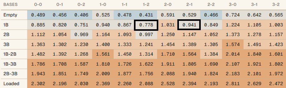
Pretty simple, right? Due to the batter winning the challenge, their team is now expected to score an extra 0.163 runs this half inning. Next lets talk about the cost of losing a challenge.
Opportunity Cost
ABS Challenges are a finite resource. Each team starts with 2 and only loses them on unsuccessful challenges. If a team enters a new extra inning and has 0, they get bumped up to 1. Only pitchers, catchers, and batters can challenge pitches. We want to quantify what losing a challenge costs you in run expectancy. Since we don't have enough historical data to get any accuracy from an empirical calculation or a simulated model, we're going to do so in a roundabout way that requires 3 simple inputs.
-
How many challenges is the team no longer going to be able to make due to losing this challenge? To get that, we need to know how many challenges the team expected to use from now until the end of the game.
-
What is the average run value of a successful challenge?
-
How often are teams correct when challenging?
Opportunity cost inputs
Number of challenge opportunities the team won't be able to make due to losing this one
As of this post, Spring Training games are averaging 4.52 ABS challenges. That's 2.26 per team per 54 outs and 0.042 per team per 1 out. When a team loses a challenge they either go from having 2 to 1 or from 1 to 0. The calculation that we run to determine how many challenges they're expected to miss out on for the rest of the game needs to account for this
Lets say a team loses their 1st challenge in the top of the 1st inning with 2 outs. They've still got 52 outs to go in the game and are expected to challenge 0.042 times per out, or 2.184 times throughout the rest of the game. How many of those are they going to miss?
For each future opportunity, the team either wins the challenge (as of this post, that's 51.7% of the time) or loses it (48.3%, burning one). Walking through all the possible sequences, a team with 2 challenges would miss about 0.04 opportunities. A team with 1 challenge would miss about 0.62. That's a difference of 0.58 extra missed opportunities you can't tap your dome for.
Average run value of a successful challenge
0.181 runs.
Challenge success rate
51.7%
Putting it all together for this example: 0.58 extra missed opportunities x 0.181 runs x 51.7% winrate = 0.053 runs
If you lose both of your challenges in the top of the 1st inning, on average, it's going to be a lot worse for your team than if you lose them towards the end of the game. You're expected to see more pitches that you want to challenge the longer the game has left.
There are a couple assumptions baked into this method that I plan on taking a look at later on: Who is the umpire, and how often are they being challenged? How many outs remain on the offensive side and the defensive side, and how often are teams challenging and winning from each? I think the way I've got this right now is generating a good context neutral approximation so we'll save that for a later date.
Lets finish off our example from earlier where instead of winning the challenge, the batter loses the challenge:
Example: Batter challenges a called strike
Runner on 1B, 0 out, 1-1 count, 1 challenge remaining. Umpire calls strike (making it 1-2). Batter challenges and loses, the call stands at 1-2, and the team loses future challenge value
Umpire's call
Opportunity cost breakdown
and now to put it all in one image:
Example: Batter challenges a called strike
Runner on 1B, 0 out, 1-1 count, 1 challenge remaining. Umpire calls strike (making it 1-2). Batter challenges. If overturned, the count becomes 2-1 instead.
Umpire's call
If overturned
Won
+0.163
If upheld — opportunity cost
Challenge Breakeven Costs
This brings us to our final topic, a concept recently published by Tom Tango. How confident do you need to be in order to challenge a call?
Here's the version that he talks about in his recent discussion that I'm going to refer to as 'unadjusted' because it assumes:
- All challenges cost the same amount at any point in the game, that is, the value of a winning challenge
- That losing a challenge with 2 remaining is the same as losing a challenge with 1 remaining
To come up with a breakeven confidence level he uses [cost / (cost + potential gain from winning)]. My run value is different because I'm making this post a bit after his, but the math is the same:
Unadjusted Challenge Breakeven Chart
Minimum probability of overturn to justify a challenge · Avg cost: 0.181 runs
Each cell shows the minimum confidence you need that a call will be overturned to justify using a challenge. Lower values (blue) mean the challenge is easier to justify because the RE swing from overturning is large relative to the cost.
| Bases | 0-0 | 0-1 | 0-2 | 1-0 | 1-1 | 1-2 | 2-0 | 2-1 | 2-2 | 3-0 | 3-1 | 3-2 |
|---|---|---|---|---|---|---|---|---|---|---|---|---|
| Empty | 73% | 72% | 52% | 62% | 65% | 47% | 48% | 51% | 38% | 43% | 36% | 23% |
| 1B | 60% | 61% | 42% | 52% | 53% | 36% | 39% | 41% | 27% | 32% | 27% | 16% |
| 2B | 62% | 59% | 36% | 54% | 55% | 33% | 44% | 44% | 27% | 47% | 36% | 18% |
| 3B | 65% | 64% | 38% | 60% | 55% | 34% | 50% | 49% | 28% | 38% | 33% | 18% |
| 1B-2B | 52% | 50% | 32% | 41% | 42% | 28% | 29% | 28% | 21% | 28% | 21% | 12% |
| 1B-3B | 64% | 57% | 29% | 49% | 50% | 26% | 37% | 44% | 23% | 32% | 27% | 14% |
| 2B-3B | 53% | 59% | 33% | 46% | 50% | 29% | 43% | 40% | 24% | 47% | 35% | 16% |
| Loaded | 51% | 44% | 26% | 40% | 37% | 23% | 30% | 29% | 17% | 21% | 18% | 10% |
Tap a cell to see details
Originally published by Tom Tango: cost-benefit analysis of making an ABS challenge.
If we adjust for the number of challenges and number of outs remaining in the game and recreate this chart, we get this:
Adjusted Challenge Breakeven Chart
Breakeven % adjusted for game timing and challenges remaining
The cost of losing a challenge depends on how many future challenge opportunities you'll miss by depleting your supply. Early in the game with one challenge left, the cost is high. Late in the game, it approaches zero. This table adjusts the breakeven confidence threshold accordingly.
| Bases | 0-0 | 0-1 | 0-2 | 1-0 | 1-1 | 1-2 | 2-0 | 2-1 | 2-2 | 3-0 | 3-1 | 3-2 |
|---|---|---|---|---|---|---|---|---|---|---|---|---|
| Empty | 46% | 45% | 26% | 34% | 37% | 22% | 23% | 25% | 16% | 19% | 15% | 9% |
| 1B | 33% | 33% | 19% | 26% | 26% | 15% | 17% | 18% | 11% | 13% | 11% | 6% |
| 2B | 35% | 32% | 15% | 27% | 28% | 13% | 20% | 20% | 11% | 22% | 15% | 7% |
| 3B | 37% | 36% | 17% | 32% | 28% | 14% | 24% | 24% | 11% | 16% | 14% | 6% |
| 1B-2B | 26% | 24% | 13% | 18% | 19% | 11% | 11% | 11% | 8% | 11% | 8% | 4% |
| 1B-3B | 36% | 30% | 12% | 24% | 24% | 10% | 16% | 20% | 9% | 13% | 10% | 5% |
| 2B-3B | 27% | 31% | 13% | 22% | 24% | 12% | 19% | 17% | 9% | 22% | 15% | 6% |
| Loaded | 25% | 20% | 10% | 18% | 16% | 9% | 12% | 12% | 6% | 8% | 7% | 3% |
Tap a cell to see details
Data from 2026 Spring Training: 51.7% challenge win rate, 0.042 challenges per team per out.
There are some huge differences here, especially when looking later into the game with 2 challenges remaining. You can find both of these values in the tables on the website. I've listed the original unadjusted values as cBE% and the adjusted as acBE%.
I'll be updating these charts with regular season data as it comes in, so look out for a post on that.
Thanks for reading, throw me a follow on Twitter/X for more.
Nate
Originally posted at 5:06pm ET on 3/13/2026